QWT 2 – Get The Unique Values From An Excel List

QWT is a series of posts that are different from the “typical” posts that are being published in this blog. As the name implies the posts are published during the weekends (Saturday or Sunday) and their subject is quick/short tips about various applications (Excel, Power Point, AutoCAD etc.). These quick tips are accompanied with step by step instructions, as well as with a lot of pictures.

---

QWT 2: Get the unique values from an Excel list

---

Today we will see how to get the unique values from an Excel list/range using four different methods:

• Removing duplicates.
• Pivot table.
• Advanced filter.
• Array formula(s).

The sequence of the methods corresponds to the degree of difficulty, implying that the method of array formula is probably the most difficult to implement. All methods are analyzed below. In all examples we assume that the original list of employees is in the range B3:B28.

---

Removing duplicates

---

Step 1: Copy the original list to another location (for safety reasons – optional step).
Step 2:. Select a cell that is included in the list.
Step 3: Go to Data tab and press the Remove Duplicates icon.

Step 4: In the pop up window:

1. Check the checkbox My data has headers (here has). 
2. Check the desired Columns.
3. Finally, press the OK button.

Step 5: A message will inform you about how many duplicate values were found and deleted.

---

Pivot table

---

Step 1: Select a cell that is included in the list.
Step 2: Go to Insert tab and press the Pivot Table icon.

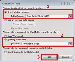
Step 3:  In the Create Pivot Table window:

1. In the Choose data you want to analyze field select the input range, if is not already selected (here ‘Pivot Table’!$B$3:$B$28).
2. In the Choose where you want the Pivot Table report to be placed, select Existing Worksheet and specify the Location you want to store the Pivot Table (here ‘Pivot Table’!$D$3).
3. Press the OK button.

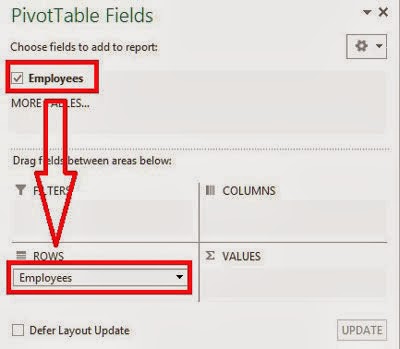
Step 4: In the Pivot Fields window select Employees and move it to the Rows field..

---

Advanced filter

---

Step 1: Select a cell that is included in the list.
Step 2: Go to Data tab and press the Advanced (filter) icon.

Step 3: In the Advanced Filter window:

1. Select the Copy to another location option.
2. Specify your data in the List range (here ‘Advanced Filter’!$B$3:$B$28). The heading (Employees) should be included in the selected List range.
3. Check the Unique records only checkbox.
4. Specify the output location at Copy to (here ‘Advanced Filter’!$D$3).
5. Press the OK button.

Step 4: A list with all the unique values will be created in the location you specified.

---

Array formula(s)

---

Step 1: Select an empty range with the same rows with your original list (here D4:D28).

Step 3: When you finish typing, don’t press ENTER, but CTRL + SHIFT + ENTER. Notice the brackets {} in the formula, implying an array formula.
Step 4: The empty range will be filled with the unique values of the initial range (here D4:D17), while #NUM! errors will appear in the rest of the cells (here D18:D28).

If you want to avoid the #NUM! errors in the range, use the IFERROR function:
Step 1: Select an empty range with the same rows with your original list (here F4:F28).

Step 3: When you finish typing, don’t press ENTER, but CTRL + SHIFT + ENTER. Notice the brackets {} in the formula, implying an array formula.
Step 4: The empty range will be filled with the unique values of the initial range (here F4:F17), while the rest of the cells will be empty (here F18:F28).

In both formulas you can use defined names instead of ranges.