About the Quick Weekend Tips (QWT) post series
QWT 1: Create an Excel chart with dynamic data range
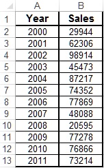
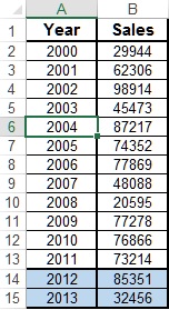
Today we will see how to create an Excel chart with dynamic data input. The tip is based on OFFSET formula and on defined names. For simplicity reasons assume that you have the following annual sales data in the range A1:B13 of Sheet1.
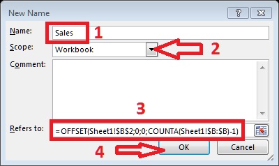
Step 1: First we will create two name ranges, “Years” and “Sales”. In the Formulas tab, select the Define Name dropdown list and select the Define Name… option.
Step 2: In the New Name form enter in the Name textbox the word “Years”, leave the dropdown list in Scope to Workbook, enter the following formula to Refers to field: =OFFSET(Sheet1!$A$2;0;0;COUNTA(Sheet1!$A:$A)-1) and press the OK button. If you receive an error while entering the formula change the “;” with “,” (this is related with the Windows regional settings of your computer). If the sheet’s name is other than “Sheet1”, change the formula accordingly – i.e. =OFFSET(Data!$A$2;0;0;COUNTA(Data!$A:$A)-1). Note the use of “!” after the sheet’s name.
Step 3: Repeat step 1 and 2, but in the Name textbox enter the word “Sales”, while to the Refers to field enter the formula: =OFFSET(Sheet1!$B$2;0;0;COUNTA(Sheet1!$B:$B)-1). Again, if the sheet’s name is other than “Sheet1”, adjust the formula accordingly.
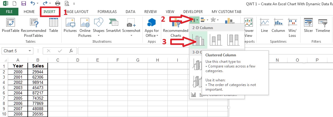
Step 4: Since we defined the necessary ranges we are now ready to create the chart. In the Insert tab, select the Insert Column chart dropdown list and select a 2-D Clustered Column chart. Of course you can select any chart type you like. The new chart will be empty.
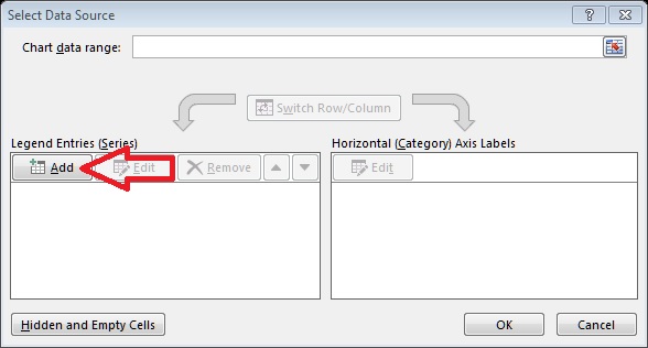
Step 5: Right click on chart and click the Select Data… option on the menu.
Step 6: In the Select Data Source form press the Add button.
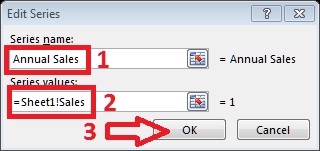
Step 7: In the Edit Series form enter the Series name (optional) – here the “Annual Sales” is used – and fill the Series values with the following formula: =Sheet1!Sales (or alternatively: Workbook Name.xlsx!Sales). Similar to steps 2 and 3, if the sheet’s name is other than “Sheet1”, change the formula accordingly. Finally, press the OK button.
Step 8: In the Select Data Source form press the Edit button.
Step 9: In the Axis Labels form fill the Axis label range with the following formula: =Sheet1!Years (or alternatively: Workbook Name.xlsx!Years) and press the OK button.
Step 10: Finally, in the Select Data Source form press the OK button.
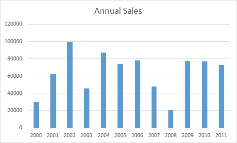
If you have completed the previous steps successfully your chart will look like this.
And here is the “fun” part. If we enter new data in the next rows of the input data, for example in the range A14:B15:
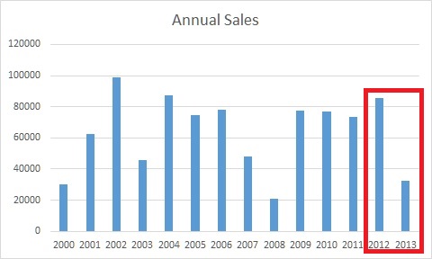
The chart automatically will show the new data:
I have used this technique in an older post, although I didn’t analyze then the way it was done..


